Load necessary packages
We first load R packages required for the example here.
library(patchwork)
library(ggtree)

# spatialCCC package
library(spatialCCC)
#> Warning: replacing previous import 'S4Arrays::makeNindexFromArrayViewport' by
#> 'DelayedArray::makeNindexFromArrayViewport' when loading 'SummarizedExperiment'
#> Warning: replacing previous import 'S4Arrays::makeNindexFromArrayViewport' by
#> 'DelayedArray::makeNindexFromArrayViewport' when loading 'HDF5Array'
Ligand-Receptor Database
Load built-in LRdb
This LRdb is downloaded from CellTalkDB: [http://tcm.zju.edu.cn/celltalkdb/download.php]. You can see the detail by:
?LRdb_human
?LRdb_mouse
We also created getter functions, get_LRdb() and get_LRdb_small(), to retrieve the database.
set.seed(100)

LRdb_m <-
  get_LRdb("mouse", n_samples = 100)

LRdb_m %>%
  dplyr::arrange(ligand_gene_symbol, receptor_gene_symbol)
#> # A tibble: 100 × 10
#>    LR    ligand_gene_symbol receptor_gene_symbol ligand_gene_id receptor_gene_id
#>    <chr> <chr>              <chr>                         <dbl>            <dbl>
#>  1 Adam… Adam10             Notch1                        11487            18128
#>  2 Adam… Adam12             Epha1                         11489            13835
#>  3 Adam… Adam17             Aplp2                         11491            11804
#>  4 Adam… Adam2              Itgb7                         11495            16421
#>  5 Adcy… Adcyap1            Adcyap1r1                     11516            11517
#>  6 Adcy… Adcyap1            Ramp3                         11516            56089
#>  7 Adip… Adipoq             Adipor1                       11450            72674
#>  8 Adm2… Adm2               Calcrl                       223780            54598
#>  9 Apoe… Apoe               Ldlr                          11816            16835
#> 10 Apoe… Apoe               Trem2                         11816            83433
#> # ℹ 90 more rows
#> # ℹ 5 more variables: ligand_ensembl_protein_id <chr>,
#> #   receptor_ensembl_protein_id <chr>, ligand_ensembl_gene_id <chr>,
#> #   receptor_ensembl_gene_id <chr>, evidence <chr>
Load Visium spatial transcriptomic data
data_dir <- spatialCCC_example("example")

spe_brain <-
  SpatialExperiment::read10xVisium(samples = data_dir,
                                   type = "HDF5",
                                   data = "filtered")

# to keep track of cell IDs
# spe_brain[["cell_id"]] <- colnames(spe_brain)

# Log-Normalize
spe_brain <- scater::logNormCounts(spe_brain)
Cell cluster data
Now, let’s read cell cluster data, obtained using GraphST.
cell_clusters <-
  read.csv(file.path(data_dir, "outs", "graphST.csv"), row.names = 1)

# Make sure the rows of cell_clusters are in the same order of spe_brain.
cell_clusters <- cell_clusters[colnames(spe_brain), ]

cluster_ids <- colnames(cell_clusters)
cluster_ids <- cluster_ids[grep("mclust_", cluster_ids)]

for (cid in cluster_ids) {
  spe_brain[[cid]] <- factor(cell_clusters[[cid]])
}
plot_spatial_feature(spe = spe_brain, feature = "mclust_8")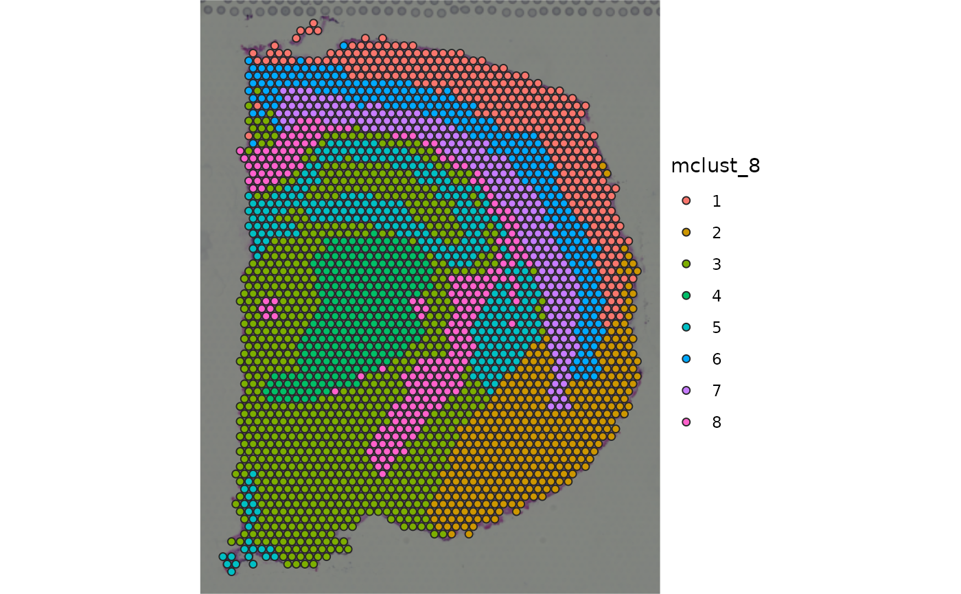
Compute Cell-Cell Communications over ligand-receptor pairs
tictoc::tic()

ccc_graph_list <-
  compute_spatial_ccc_graph_list(spe = spe_brain,
                                 assay_name = "logcounts",
                                 LRdb = LRdb_m)

tictoc::toc()
#> 694.279 sec elapsed
ccc_graph_list <-
  ccc_graph_list %>%
  purrr::map(function(ccog) {
    ccog %>%
      add_node_annot_to_edges(c("mclust_8", "mclust_9", "mclust_10"))
  })
ccc_tbl <-
  ccc_graph_list %>%
  purrr::map(function(ccog) {
    ccog %>%
      tidygraph::activate("edges") %>%
      as_tibble()
  }) %>%
  dplyr::bind_rows(.id = "LR")
Summarize cell-cell communication between cell clusters
ccc_tbl_between_clusters <-
  ccc_tbl %>%
  dplyr::group_by(mclust_8_src, mclust_8_dst, LR) %>%
  dplyr::summarise(n = dplyr::n(),
                   LRscore.sum = sum(LRscore),
                   .groups = "drop")

ccc_tbl_between_clusters %>%
  dplyr::arrange(desc(n))
#> # A tibble: 1,327 × 5
#>    mclust_8_src mclust_8_dst LR                    n LRscore.sum
#>    <fct>        <fct>        <chr>             <int>       <dbl>
#>  1 3            3            App_Lrp1           4480       3576.
#>  2 3            3            Nlgn2_Nrxn1        3592       2585.
#>  3 3            3            Ncam1_Fgfr1        3093       2167.
#>  4 3            3            S100a1_Ryr2        2349       1592.
#>  5 2            2            App_Lrp1           2136       1710.
#>  6 3            3            Apoe_Ldlr          1953       1487.
#>  7 2            2            Nlgn2_Nrxn1        1840       1386.
#>  8 1            1            App_Lrp1           1742       1406.
#>  9 3            3            Apoe_Trem2         1720       1322.
#> 10 3            3            Adcyap1_Adcyap1r1  1687       1131.
#> # ℹ 1,317 more rows
ccc_tbl_between_clusters %>%
  dplyr::filter(mclust_8_dst != mclust_8_src) %>%
  dplyr::arrange(desc(n))
#> # A tibble: 1,004 × 5
#>    mclust_8_src mclust_8_dst LR                n LRscore.sum
#>    <fct>        <fct>        <chr>         <int>       <dbl>
#>  1 3            5            App_Lrp1        304        241.
#>  2 5            3            App_Lrp1        300        238.
#>  3 5            3            Nlgn2_Nrxn1     255        184.
#>  4 3            5            S100a1_Ryr2     224        161.
#>  5 8            3            App_Lrp1        212        171.
#>  6 3            5            Ncam1_Fgfr1     208        145.
#>  7 3            8            App_Lrp1        199        157.
#>  8 3            5            Nlgn2_Nrxn1     195        141.
#>  9 5            3            Ncam1_Fgfr1     165        116.
#> 10 3            5            Calm2_Cacna1c   163        122.
#> # ℹ 994 more rows
Convert CCC table to CCC graph
summarize_ccc_graph_metrics() summarize those graph metrics for each LR pair.
tictoc::tic()

ccc_graph_metrics_summary_df <-
  summarize_ccc_graph_metrics(ccc_graph_list)

tictoc::toc()
#> 0.237 sec elapsed
ccc_graph_metrics_summary_df %>%
  dplyr::arrange(graph_component_count)
#> # A tibble: 41 × 12
#>    LR        graph_n_nodes graph_n_edges graph_component_count graph_motif_count
#>    <chr>             <int>         <dbl>                 <dbl>             <int>
#>  1 App_Lrp1           2700         17430                     3             27811
#>  2 Ncam1_Fg…          2549          9640                     3             18340
#>  3 Nlgn2_Nr…          2675         14289                     3             25062
#>  4 S100a1_R…          2591         10689                     5             20094
#>  5 Calm2_Ca…          2461          8105                     6             16288
#>  6 Apoe_Tre…          2560          6937                     8             14484
#>  7 Apoe_Ldlr          2295          5608                    26             11724
#>  8 Slit1_Ro…          1651          4373                    41              7866
#>  9 Calm2_My…          1967          4247                    42              8830
#> 10 Adcyap1_…          1642          4172                    43              7801
#> # ℹ 31 more rows
#> # ℹ 7 more variables: graph_diameter <dbl>, graph_un_diameter <dbl>,
#> #   graph_mean_dist <dbl>, graph_circuit_rank <dbl>, graph_reciprocity <dbl>,
#> #   graph_clique_num <int>, graph_clique_count <int>
summarize_ccc_graph_metrics(…, level = “group”) summarizes the metrics for each subgraph (group) in CCC graph (LR)
tictoc::tic()

ccc_graph_group_metrics_summary_df <-
  summarize_ccc_graph_metrics(ccc_graph_list, level = "group")

tictoc::toc()
#> 0.305 sec elapsed
ccc_graph_group_metrics_summary_df
#> # A tibble: 2,877 × 12
#>    LR         group group_n_nodes group_n_edges group_adhesion group_motif_count
#>    <chr>      <int>         <int>         <dbl>          <dbl>             <int>
#>  1 Rspo3_Lgr6    38             2             1              0                 0
#>  2 Rspo3_Lgr6    13             3             3              0                 1
#>  3 Rspo3_Lgr6    39             2             1              0                 0
#>  4 Rspo3_Lgr6    14             3             2              0                 1
#>  5 Rspo3_Lgr6     5             4             3              0                 3
#>  6 Rspo3_Lgr6     6             4             4              0                 3
#>  7 Rspo3_Lgr6    75             1             1              0                 0
#>  8 Rspo3_Lgr6    40             2             1              0                 0
#>  9 Rspo3_Lgr6    41             2             1              0                 0
#> 10 Rspo3_Lgr6    15             3             3              0                 1
#> # ℹ 2,867 more rows
#> # ℹ 6 more variables: group_diameter <dbl>, group_un_diameter <dbl>,
#> #   group_mean_dist <dbl>, group_girth <dbl>, group_circuit_rank <dbl>,
#> #   group_reciprocity <dbl>
Visualization
LR_of_interest <- "Pdgfb_Pdgfra"
ccc_graph_list[[LR_of_interest]] %>%
  tidygraph::activate(edges) %>%
  tibble::as_tibble()
#> # A tibble: 2,406 × 40
#>     from    to src    dst       d norm.d ligand receptor LRscore weight WLRscore
#>    <int> <int> <chr>  <chr> <dbl>  <dbl> <chr>  <chr>      <dbl>  <dbl>    <dbl>
#>  1     1     1 AAACA… AAAC…    0    0    Pdgfb  Pdgfra     0.621  1        0.621
#>  2     1   920 AAACA… AGAG…  138.   1.01 Pdgfb  Pdgfra     0.649  0.980    0.636
#>  3     1   921 AAACA… GGCA…  138.   1.01 Pdgfb  Pdgfra     0.684  0.987    0.675
#>  4     1   896 AAACA… TTCT…  138.   1.01 Pdgfb  Pdgfra     0.629  0.980    0.616
#>  5     2   922 AAACA… TCAC…  138.   1.01 Pdgfb  Pdgfra     0.599  0.980    0.587
#>  6     3     3 AAACC… AAAC…    0    0    Pdgfb  Pdgfra     0.541  1        0.541
#>  7     3   923 AAACC… CGCT…  138    1.01 Pdgfb  Pdgfra     0.631  0.986    0.622
#>  8     3   924 AAACC… TTGG…  138.   1.01 Pdgfb  Pdgfra     0.509  0.980    0.498
#>  9     4     4 AAACG… AAAC…    0    0    Pdgfb  Pdgfra     0.641  1        0.641
#> 10     4    50 AAACG… AAGA…  138    1.01 Pdgfb  Pdgfra     0.670  0.986    0.660
#> # ℹ 2,396 more rows
#> # ℹ 29 more variables: LRscore_perc_rank <dbl>, graph_n_nodes <int>,
#> #   graph_n_edges <dbl>, graph_component_count <dbl>, graph_motif_count <int>,
#> #   graph_diameter <dbl>, graph_un_diameter <dbl>, graph_mean_dist <dbl>,
#> #   graph_circuit_rank <dbl>, graph_reciprocity <dbl>, graph_clique_num <int>,
#> #   graph_clique_count <int>, group <int>, group_n_nodes <int>,
#> #   group_n_edges <dbl>, group_adhesion <dbl>, group_motif_count <int>, …
spatial CCC graph plot with tissue image
gp_spccc <-
  plot_spatial_ccc_graph(
    ccc_graph = ccc_graph_list[[LR_of_interest]],
    tissue_img = SpatialExperiment::imgRaster(spe_brain),
    node_color = "mclust_8",
    node_size = 1,
    node_alpha = 0.5,
    edge_color = "group",
    # clip = TRUE,
    which_on_top = "edge"
  )

gp_spccc_0 <-
  plot_spatial_feature(spe = spe_brain,
                       feature = "mclust_8")
wrap_plots(gp_spccc, gp_spccc_0, ncol = 2)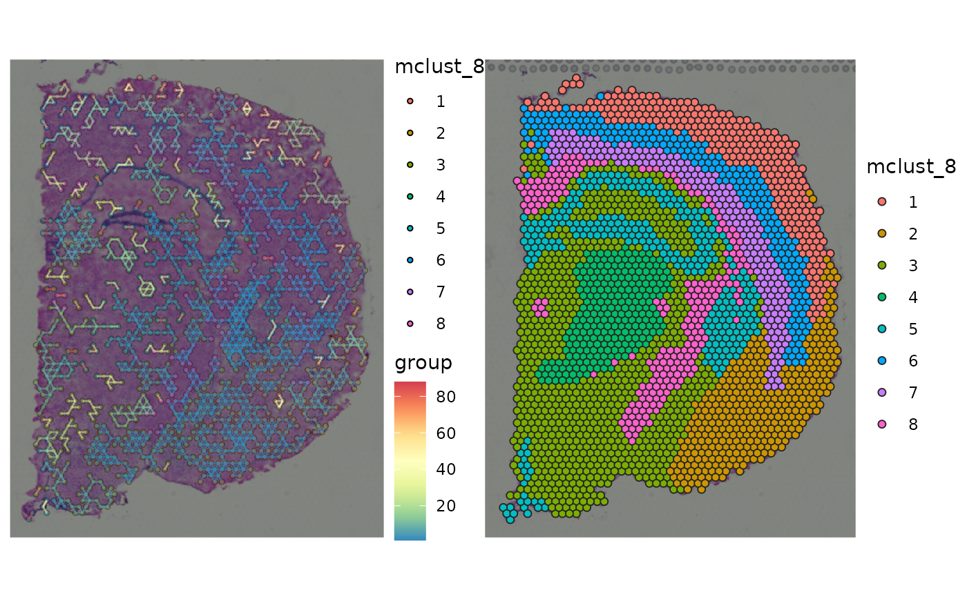
ccc_graph_temp <-
  ccc_graph_list[[LR_of_interest]] %>%
  tidygraph::activate("edges") %>%
  tidygraph::filter(mclust_8_src != mclust_8_dst) %>%
  tidy_up_ccc_graph()

cells_of_interest <-
  ccc_graph_temp %>%
  tidygraph::activate("nodes") %>%
  dplyr::pull("name")
gp_spccc <-
  plot_spatial_ccc_graph(
    ccc_graph = ccc_graph_temp,
    tissue_img = SpatialExperiment::imgRaster(spe_brain),
    node_color = "n.inflow",
    node_size = 1.25,
    node_alpha = 1,
    edge_color = "group",
    show_arrow = TRUE,
    # clip = TRUE,
    which_on_top = "node"
  )

gp_spccc_0 <-
  plot_spatial_ccc_graph(
    ccc_graph = ccc_graph_list[[LR_of_interest]],
    tissue_img = SpatialExperiment::imgRaster(spe_brain),
    image_alpha = 0,
    cells_of_interest = cells_of_interest,
    edges_expanded_to_group = FALSE,
    node_color = "mclust_8",
    node_size = 1.25,
    node_alpha = 0.5,
    edge_color = "group",
    show_arrow = TRUE,
    # clip = TRUE,
    which_on_top = "node"
  )

gp_spccc_1 <-
  plot_spatial_feature(spe = spe_brain,
                       feature = "mclust_8",
                       cells_of_interest = cells_of_interest)
wrap_plots(gp_spccc, gp_spccc_1, ncol = 2)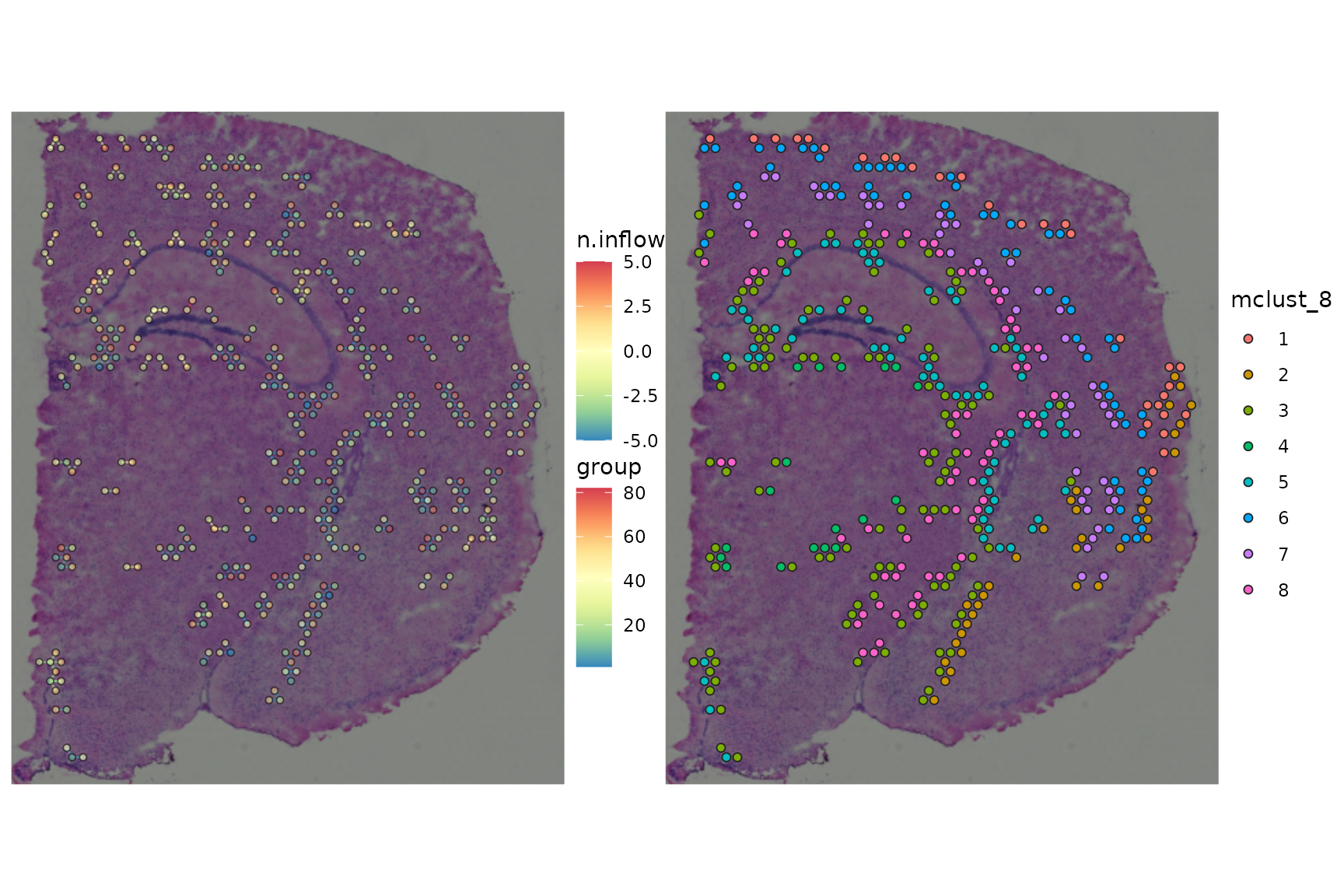
gp_spccc_0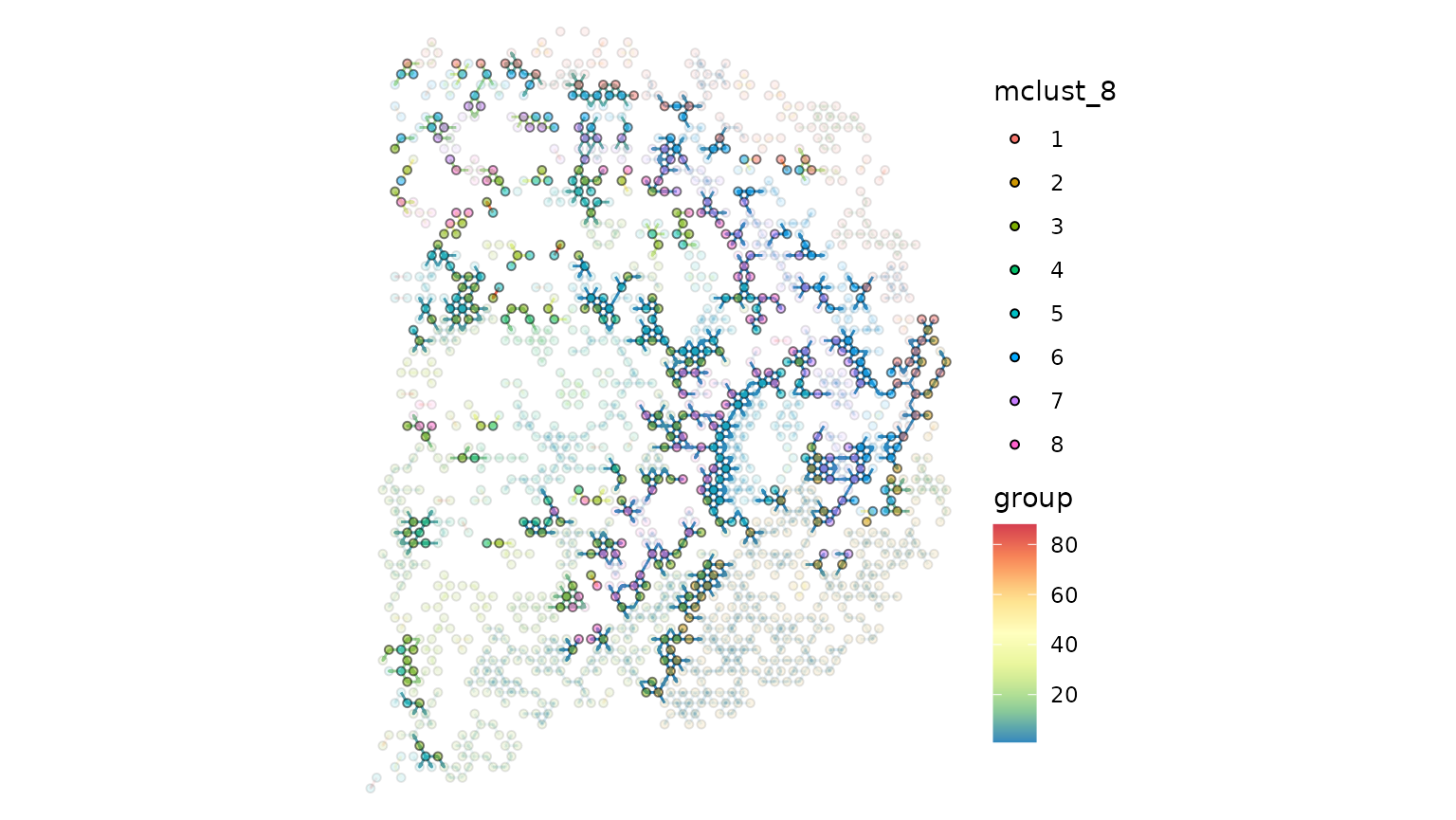
spatial CCC graph plot without tissue image
In this case, graph layout can be “spatial” which keeps the original spatial locations, or other graph layout algorithm supported by igraph package.
gp_spccc <-
  plot_spatial_ccc_graph(
    ccc_graph = ccc_graph_list[[LR_of_interest]],
    graph_layout = "spatial",
    node_color =  "mclust_8",
    node_size = 1,
    edge_color = "group_diameter",
    clip = TRUE,
    # ghost_img = TRUE,
    which_on_top = "edge"
  )

gp_spccc_0 <-
  plot_spatial_ccc_graph(
    ccc_graph =
      ccc_graph_list[[LR_of_interest]],
    graph_layout = "spatial",
    node_color = "mclust_8",
    node_size = 1,
    edge_color = "group_diameter",
    clip = TRUE,
    # ghost_img = TRUE,
    which_on_top = "node"
  )
wrap_plots(gp_spccc, gp_spccc_0, ncol = 2, guides = "collect")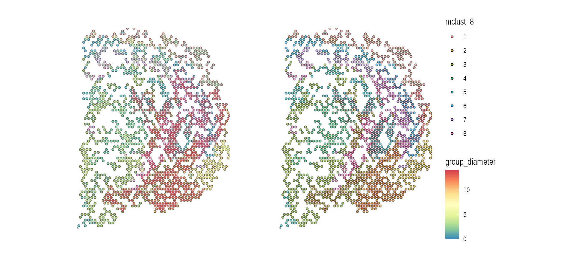
Below uses “auto” layout (“kk” spring layout).
plot_spatial_ccc_graph(ccc_graph = ccc_graph_list[[LR_of_interest]],
                       # tissue_img = SpatialExperiment::imgRaster(spe_brain),
                       node_color = "group",
                       node_size = 0.1,
                       edge_color = "group_diameter",
                       edge_width = 0.1,
                       which_on_top = "edge")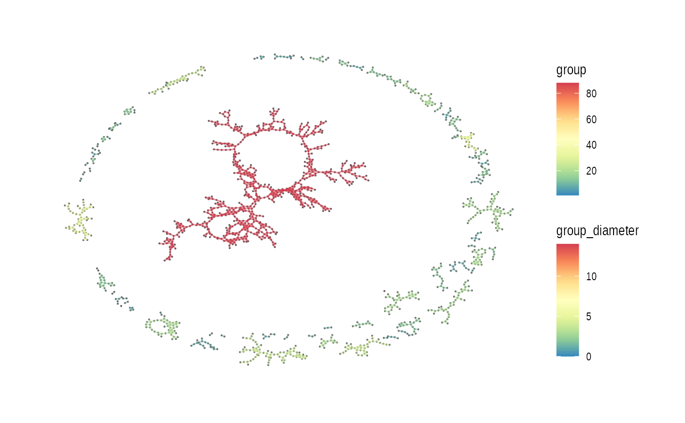
In this case, below is “stress” layout.
plot_spatial_ccc_graph(ccc_graph = ccc_graph_list[[LR_of_interest]],
                       # tissue_img = SpatialExperiment::imgRaster(spe_brain),
                       graph_layout = "stress",
                       node_color = "group",
                       edge_color = "group_diameter",
                       edge_width = 0.25,
                       which_on_top = "edge")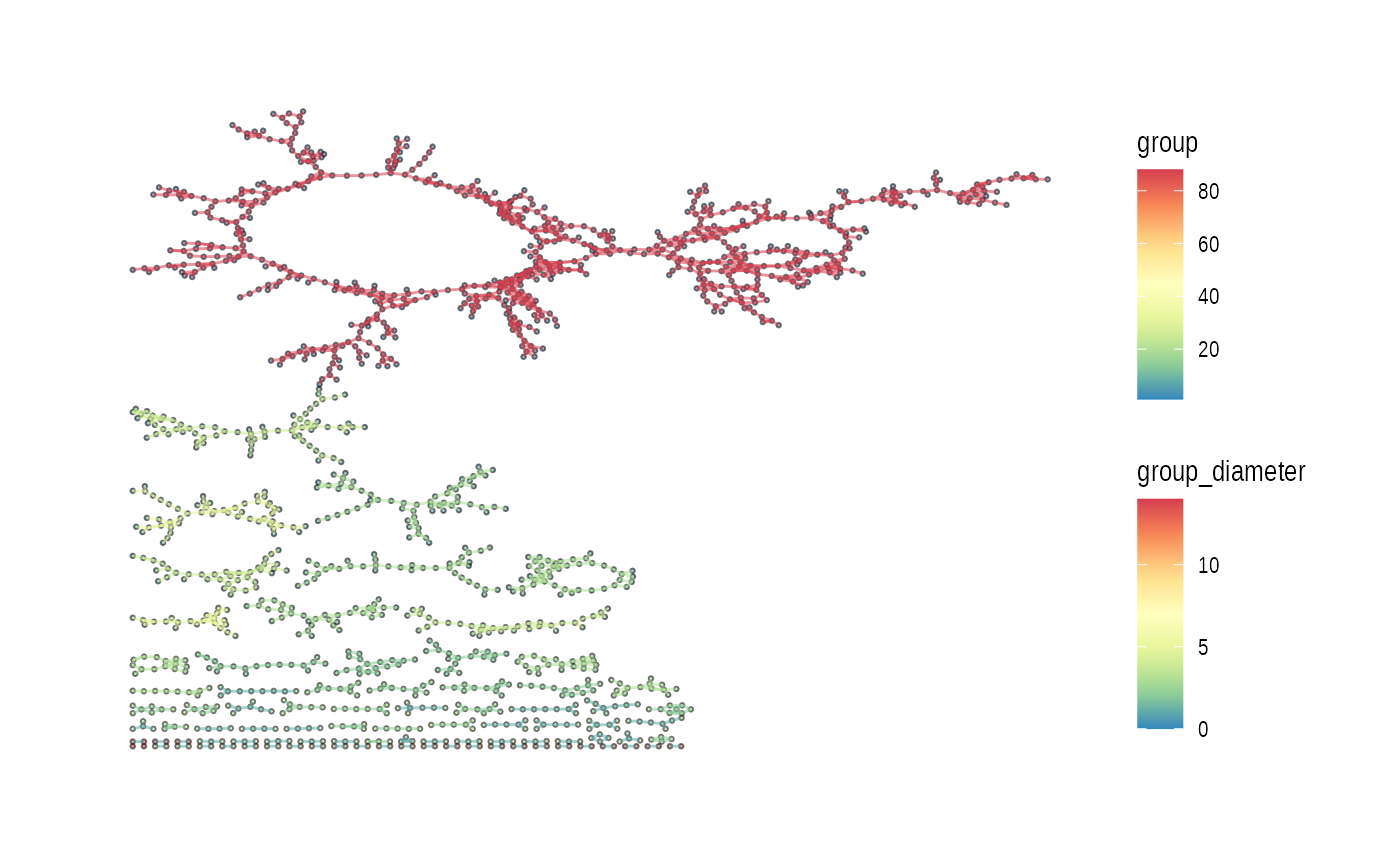
Cell-overlap distance
tictoc::tic()

cell_overlap_dist <-
  dist_cell_overlap_ccc_tbl(ccc_tbl)

tictoc::toc()
#> 0.878 sec elapsed
tictoc::tic()

cell_overlap_lf <-
  lf_cell_overlap_ccc_tbl(ccc_tbl)

tictoc::toc()
#> 1.229 sec elapsed
tictoc::tic()

LRs_high_cell_overlap <-
  cell_overlap_lf %>%
  dplyr::filter(d < 1) %>%
  dplyr::select(lr1, lr2) %>%
  unlist() %>% unique()

tictoc::toc()
#> 0.011 sec elapsed
tictoc::tic()

high_cell_overlap_dist <-
  cell_overlap_dist[LRs_high_cell_overlap, LRs_high_cell_overlap]

tictoc::toc()
#> 0.003 sec elapsed
tictoc::tic()

high_cell_overlap_dist2 <-
  cell_overlap_lf %>%
  dplyr::filter(d < 1) %>%
  dplyr::select(lr1, lr2, d) %>%
  lf_to_dist()

tictoc::toc()
#> 0.031 sec elapsed
LR_ccc_summary_tbl <-
  ccc_tbl %>%
  dplyr::pull(LR) %>%
  table() %>%
  tibble::as_tibble() %>%
  dplyr::rename("LR" = ".") %>%
  dplyr::arrange(desc(n)) %>%
  dplyr::left_join(
    ccc_tbl %>%
      dplyr::select(LR, ligand, receptor) %>%
      dplyr::distinct(),
    by = "LR"
  )
ape::as.phylo(hclus.res) %>%
  ggtree(layout="dendrogram") %<+% LR_ccc_summary_tbl +
  aes(color=receptor) +
  theme(legend.position = "none") +
  geom_tippoint(aes(size=n), alpha=0.5) +
  geom_tiplab(size=2, offset=-0.15) +
  xlim_tree(3)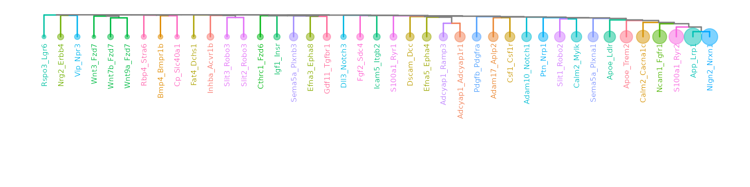
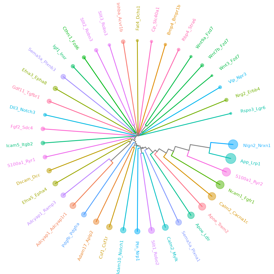
ape::as.phylo(hclus.res) %>%
  ggtree(layout = "circular") %<+% LR_ccc_summary_tbl +
  aes(color=receptor) +
  # aes(color=ligand) +
  theme(legend.position = "none") +
  geom_tippoint(aes(size=n), alpha=0.5) +
  geom_tiplab(size=2, offset=0.05)