library(spatialCCC)
#> Warning: replacing previous import 'S4Arrays::makeNindexFromArrayViewport' by
#> 'DelayedArray::makeNindexFromArrayViewport' when loading 'SummarizedExperiment'
#> Warning: replacing previous import 'S4Arrays::makeNindexFromArrayViewport' by
#> 'DelayedArray::makeNindexFromArrayViewport' when loading 'HDF5Array'
library(dplyr)
#>
#> Attaching package: 'dplyr'
#> The following objects are masked from 'package:stats':
#>
#>     filter, lag
#> The following objects are masked from 'package:base':
#>
#>     intersect, setdiff, setequal, union
library(ggplot2)
library(patchwork)- Then, load built-in LR database.
set.seed(100)

LRdb_m <-
  get_LRdb("mouse", n_samples = 100)

LRdb_full <-
  get_LRdb("mouse")

LRdb <- LRdb_m
#LRdb <- LRdb_full- Load an example Visium spatial transcriptomic data
# absolute path to "example" spatial transcriptomic data
data_dir <- spatialCCC_example("example")

spe_brain <-
  SpatialExperiment::read10xVisium(samples = data_dir,
                                   type = "HDF5",
                                   data = "filtered")

# Log-Normalize
spe_brain <- scater::logNormCounts(spe_brain)
Cell-cell communication analysis
- Compute Cell-Cell Communications over ligand-receptor pairs
#future::plan(future::multisession, workers = 8)

ccc_graph_list <-
  compute_spatial_ccc_graph_list(spe = spe_brain,
                                 assay_name = "logcounts",
                                 LRdb = LRdb)

#future::plan(future::sequential)- Summarize spatial CCC graphs by LR
ccc_graph_summary_tbl <-
  ccc_graph_list %>%
  to_LR_summary_tbl() %>%
  arrange(desc(perc_rank))

ccc_graph_summary_tbl
#> # A tibble: 41 × 20
#>    LR          L     R         n LRscore n_perc_rank LRscore_perc_rank perc_rank
#>    <chr>       <chr> <chr> <int>   <dbl>       <dbl>             <dbl>     <dbl>
#>  1 App_Lrp1    App   Lrp1  17430   0.806       1                 1         1
#>  2 Apoe_Trem2  Apoe  Trem2  6937   0.767       0.875             0.975     0.924
#>  3 Nlgn2_Nrxn1 Nlgn2 Nrxn1 14289   0.741       0.975             0.875     0.924
#>  4 Calm2_Cacn… Calm2 Cacn…  8105   0.760       0.9               0.925     0.912
#>  5 Apoe_Ldlr   Apoe  Ldlr   5608   0.764       0.85              0.95      0.899
#>  6 S100a1_Ryr2 S100… Ryr2  10689   0.690       0.95              0.825     0.885
#>  7 Ncam1_Fgfr1 Ncam1 Fgfr1  9640   0.688       0.925             0.8       0.860
#>  8 Calm2_Mylk  Calm2 Mylk   4247   0.750       0.8               0.9       0.849
#>  9 Adcyap1_Ad… Adcy… Adcy…  4172   0.644       0.775             0.75      0.762
#> 10 Adam17_Apl… Adam… Aplp2  3338   0.692       0.675             0.85      0.757
#> # ℹ 31 more rows
#> # ℹ 12 more variables: perc_group <chr>, graph_n_nodes <int>,
#> #   graph_n_edges <dbl>, graph_component_count <dbl>, graph_motif_count <int>,
#> #   graph_diameter <dbl>, graph_un_diameter <dbl>, graph_mean_dist <dbl>,
#> #   graph_circuit_rank <dbl>, graph_reciprocity <dbl>, graph_clique_num <int>,
#> #   graph_clique_count <int>
top_LR <-
  ccc_graph_summary_tbl %>%
  pull(LR) %>%
  head(n = 1)

bottom_LR <-
  ccc_graph_summary_tbl %>%
  pull(LR) %>%
  tail(n = 1)
gp_ccc_graph_top_LR <-
  plot_spatial_ccc_graph(ccc_graph_list[[top_LR]],
                         graph_layout = "spatial",
                         edge_color = "LRscore",
                         node_color = "LRscore.sum.src") +
  ggtitle(top_LR)

gp_ccc_graph_bottom_LR <-
  plot_spatial_ccc_graph(ccc_graph_list[[bottom_LR]],
                         graph_layout = "spatial",
                         edge_color = "LRscore",
                         node_color = "LRscore.sum.src") +
  ggtitle(bottom_LR)
wrap_plots(gp_ccc_graph_top_LR, gp_ccc_graph_bottom_LR)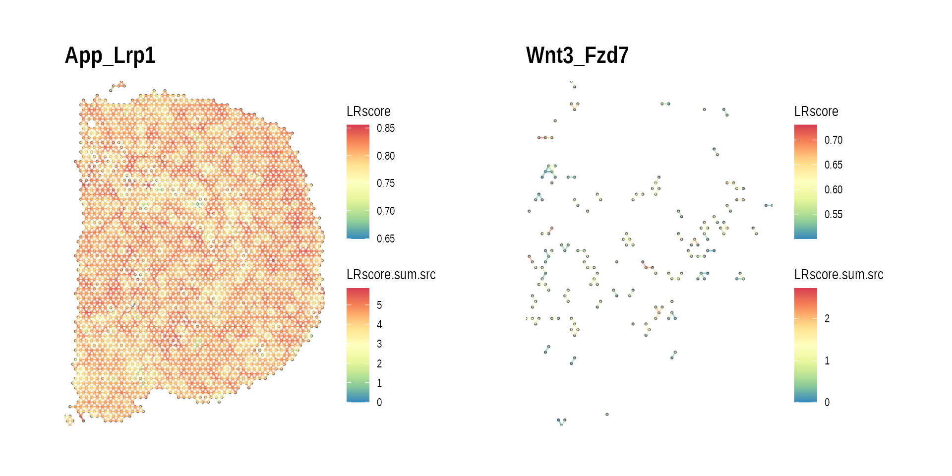
- CCC graph summary table only with ligands or receptors with multiple occurrences
L_high_freq <-
  ccc_graph_summary_tbl %>%
  group_by(L) %>%
  summarise(n = n(), .groups = "drop") %>%
  dplyr::filter(n > 1) %>%
  dplyr::arrange(desc(n)) %>%
  pull(L)

L_high_freq
#> [1] "Adcyap1" "Apoe"    "Calm2"   "S100a1"  "Sema5a"
R_high_freq <-
  ccc_graph_summary_tbl %>%
  group_by(R) %>%
  summarise(n = n(), .groups = "drop") %>%
  dplyr::filter(n > 1) %>%
  dplyr::arrange(desc(n)) %>%
  pull(R)

R_high_freq
#> [1] "Fzd7"  "Robo3"
ccc_graph_summary_tbl %>%
  dplyr::filter(L %in% L_high_freq | R %in% R_high_freq)
#> # A tibble: 15 × 20
#>    LR          L     R         n LRscore n_perc_rank LRscore_perc_rank perc_rank
#>    <chr>       <chr> <chr> <int>   <dbl>       <dbl>             <dbl>     <dbl>
#>  1 Apoe_Trem2  Apoe  Trem2  6937   0.767       0.875             0.975    0.924
#>  2 Calm2_Cacn… Calm2 Cacn…  8105   0.760       0.9               0.925    0.912
#>  3 Apoe_Ldlr   Apoe  Ldlr   5608   0.764       0.85              0.95     0.899
#>  4 S100a1_Ryr2 S100… Ryr2  10689   0.690       0.95              0.825    0.885
#>  5 Calm2_Mylk  Calm2 Mylk   4247   0.750       0.8               0.9      0.849
#>  6 Adcyap1_Ad… Adcy… Adcy…  4172   0.644       0.775             0.75     0.762
#>  7 Sema5a_Plx… Sema… Plxn…  3869   0.609       0.75              0.55     0.642
#>  8 Sema5a_Plx… Sema… Plxn…  2054   0.622       0.575             0.625    0.599
#>  9 S100a1_Ryr1 S100… Ryr1   1060   0.637       0.45              0.675    0.551
#> 10 Adcyap1_Ra… Adcy… Ramp3  2039   0.608       0.55              0.525    0.537
#> 11 Wnt7b_Fzd7  Wnt7b Fzd7    528   0.583       0.25              0.2      0.224
#> 12 Slit2_Robo3 Slit2 Robo3   687   0.578       0.325             0.125    0.202
#> 13 Wnt9a_Fzd7  Wnt9a Fzd7    193   0.566       0.075             0.025    0.0433
#> 14 Slit3_Robo3 Slit3 Robo3   263   0.557       0.15              0        0
#> 15 Wnt3_Fzd7   Wnt3  Fzd7    144   0.588       0                 0.325    0
#> # ℹ 12 more variables: perc_group <chr>, graph_n_nodes <int>,
#> #   graph_n_edges <dbl>, graph_component_count <dbl>, graph_motif_count <int>,
#> #   graph_diameter <dbl>, graph_un_diameter <dbl>, graph_mean_dist <dbl>,
#> #   graph_circuit_rank <dbl>, graph_reciprocity <dbl>, graph_clique_num <int>,
#> # graph_clique_count <int>- Spatial CCC graph with ligand with multiple occurences
high_L_LR_list <-
  ccc_graph_summary_tbl %>%
  dplyr::filter(L == L_high_freq[1]) %>%
  pull(LR) %>%
  setNames(nm = .)

gp_list <-
  high_L_LR_list %>%
  purrr::map(function(lr) {
    plot_spatial_ccc_graph(
      ccc_graph_list[[lr]],
      graph_layout = "spatial",
      edge_color = "LRscore",
      clip = FALSE
    ) +
      ggtitle(lr)
  })
wrap_plots(gp_list)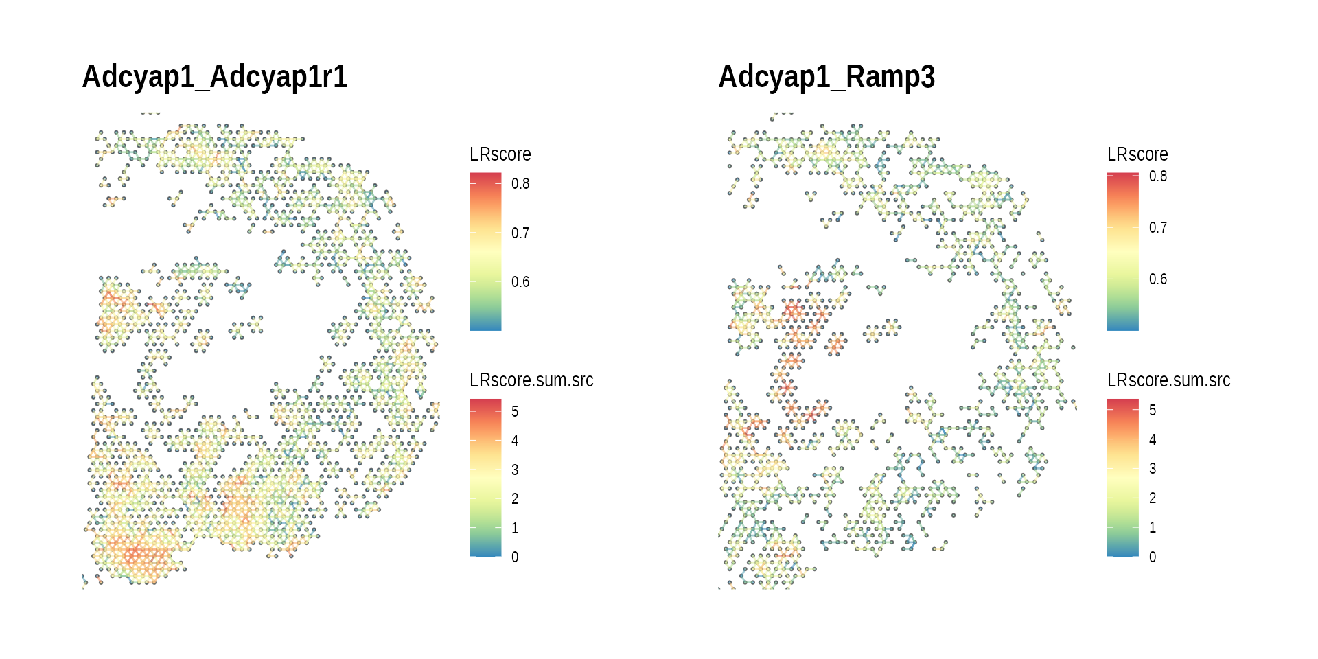
high_R_LR_list <-
  ccc_graph_summary_tbl %>%
  dplyr::filter(R == R_high_freq[1]) %>%
  pull(LR) %>%
  setNames(nm = .)

gp_list <-
  high_R_LR_list %>%
  purrr::map(function(lr) {
    plot_spatial_ccc_graph(
      ccc_graph_list[[lr]],
      graph_layout = "spatial",
      edge_color = "LRscore",
      clip = FALSE
    ) +
      ggtitle(lr)
  })
wrap_plots(gp_list)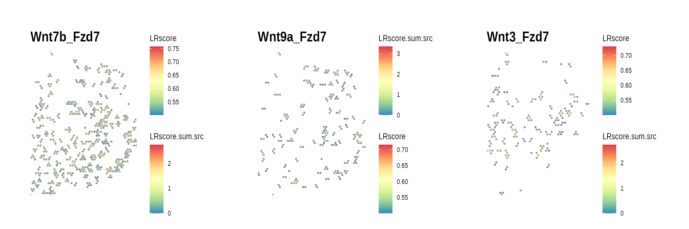
ccog_diff_1 <-
  ccc_graph_diff(ccc_graph_list[[high_L_LR_list[1]]],
                 ccc_graph_list[[high_L_LR_list[2]]])

ccog_diff_2 <-
  ccc_graph_diff(ccc_graph_list[[high_L_LR_list[2]]],
                 ccc_graph_list[[high_L_LR_list[1]]])
ccog_union <-
  ccc_graph_union(ccc_graph_list[[high_L_LR_list[1]]],
                  ccc_graph_list[[high_L_LR_list[2]]])

ccog_intersect <-
  ccc_graph_intersect(ccc_graph_list[[high_L_LR_list[1]]],
                      ccc_graph_list[[high_L_LR_list[2]]])
gp_list <-
  list(ccog_diff_1, ccog_diff_2) %>%
  purrr::map(function(ccog) {
    plot_spatial_ccc_graph(ccog,
                           graph_layout = "spatial")
  })
wrap_plots(gp_list)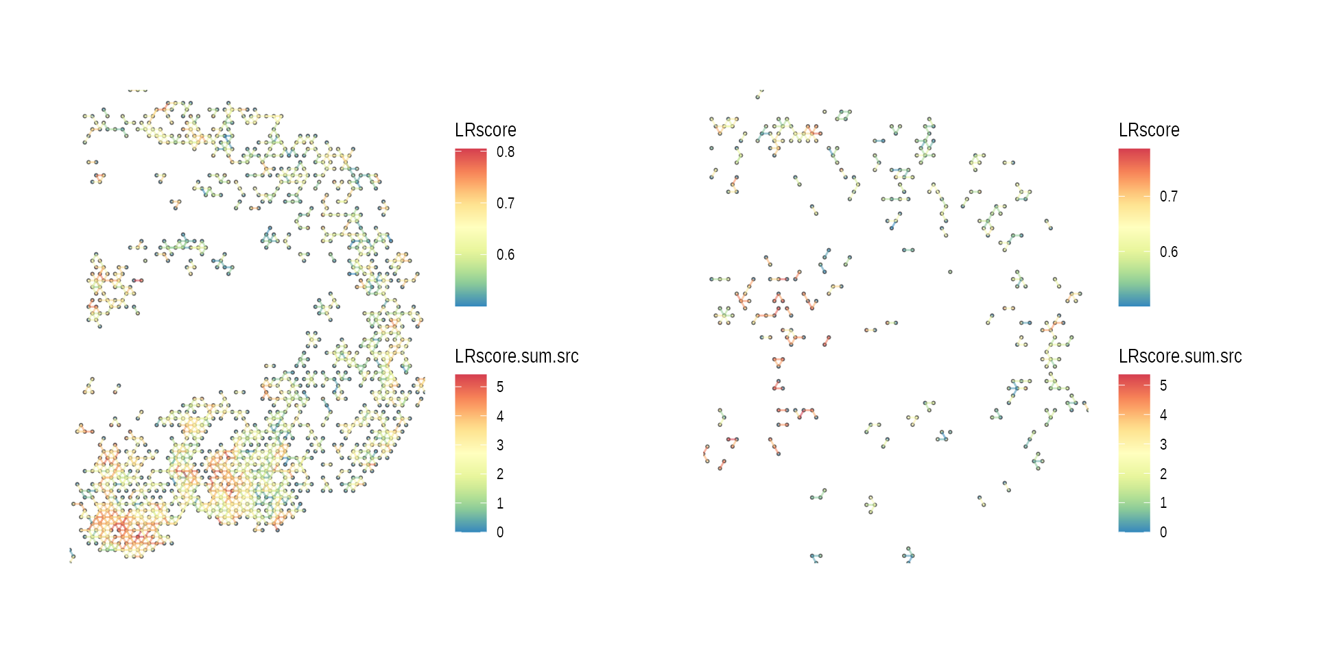
gp_list <-
  list(ccog_diff_1, ccog_diff_2) %>%
  purrr::map(function(ccog) {
    plot_spatial_ccc_graph(ccog,
                           graph_layout = "spatial")
  })
wrap_plots(gp_list)
gp_list <-
  list(intersect = ccog_intersect, union = ccog_union) %>%
  purrr::map(function(ccog) {
    plot_spatial_ccc_graph(ccog,
                           graph_layout = "spatial")
  })
wrap_plots(gp_list)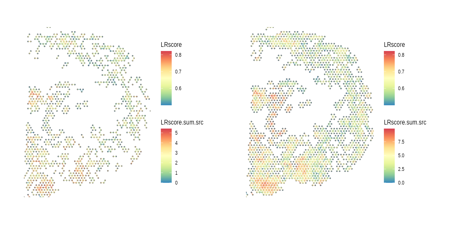
gp_list <-
  list(ccog_diff_1, ccog_diff_2) %>%
  purrr::map(function(ccog) {
    plot_spatial_ccc_graph(ccog,
                           graph_layout = "spatial",
                           tissue_img = SpatialExperiment::imgRaster(spe_brain))
  })
wrap_plots(gp_list)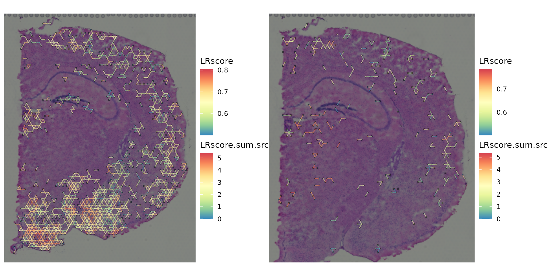
gp_list <-
  list(intersect = ccog_intersect, union = ccog_union) %>%
  purrr::map(function(ccog) {
    plot_spatial_ccc_graph(ccog,
                           graph_layout = "spatial",
                           tissue_img = SpatialExperiment::imgRaster(spe_brain))
  })
wrap_plots(gp_list)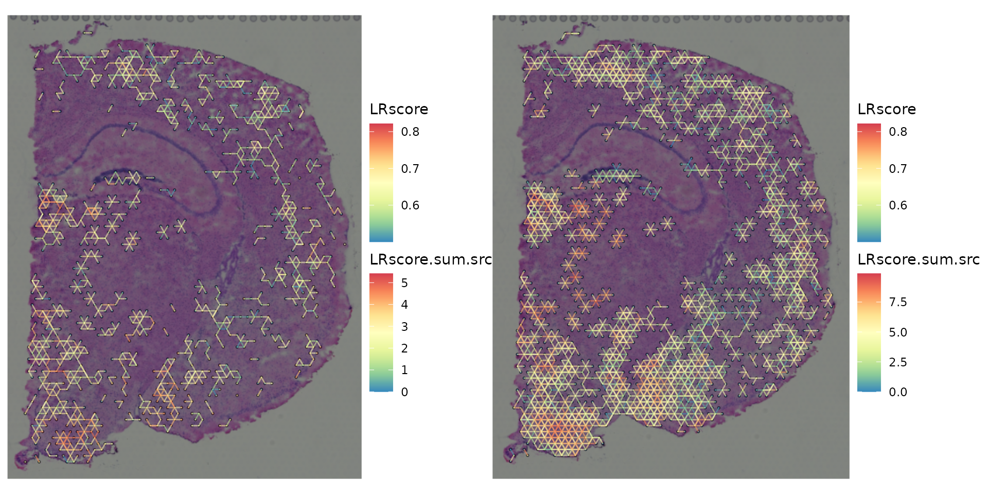
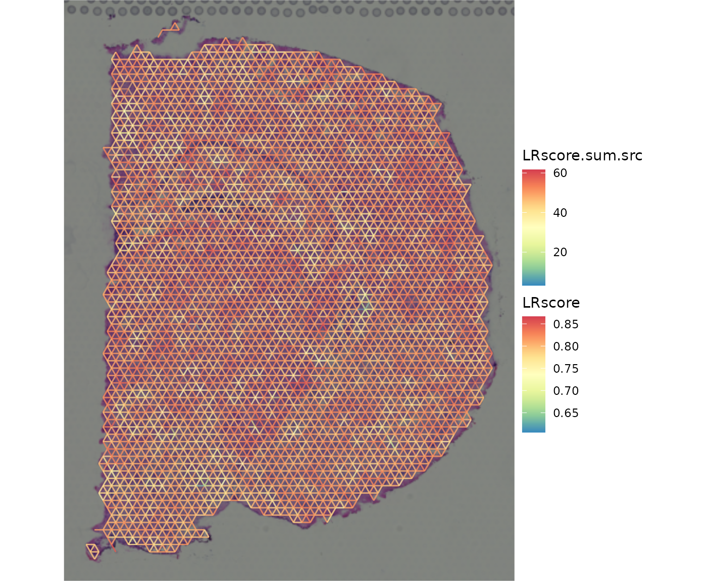
ccog_flattened <-
  flatten_ccc_graph_list(ccc_graph_ls = ccc_graph_list)
plot_spatial_ccc_graph(
  ccog_flattened,
  tissue_img = SpatialExperiment::imgRaster(spe_brain),
  graph_layout = "spatial",
  node_color = "LRscore.sum.src",
  edge_color = "LRscore",
  # node_size = 1.6,
  node_alpha = 0,
  which_on_top = "edge"
)